Benchmark: Flexibility Region Estimation Methods

Background and Motivation
See the literature review section for an overview of existing methods for estimating flexibility regions at TSO-DSO interfaces.
Method Comparison
Static Methods
Methods that estimate flexibility regions without considering the temporal dynamics of the devices like battery storage.
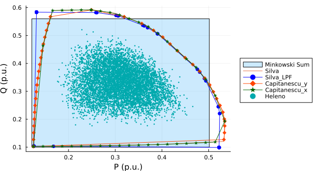
Simple Minkowski Sum
The Minkowski sum method estimates the flexibility region by summing the individual flexibility regions of each device without considering the non-linear network constraints. This method assumes that the devices operate independently and that their flexibility regions can be combined linearly.
Usually given by sector-coupling related researches, e.g. [1]
Pros:
- computationally efficient
- easy to implement
Cons:
- does not capture the interactions between devices and network constraints and thus overestimates the flexibility region
- could not capture the losses in the network
Sampling-Based Methods
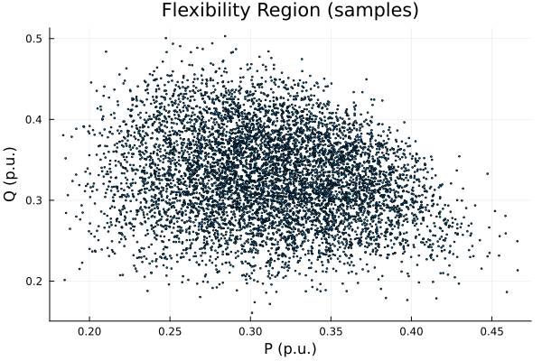
[2] propose a Monte Carlo sampling-based method to estimate the flexibility region of a distribution network. The process involves the following steps:
- generate random samples of the power injections of the flexible devices;
- check the wholistic feasibility against the network constraints via power flow calculations;
- record the feasible samples and the corresponding costs that satisfy all constraints;
- the flexibility region is then approximated by the envelope of the feasible samples.
Pros:
- straightforward to implement
- can capture non-convexities in the flexibility region
- can give the cost associated with each point in the flexibility region
Cons:
- computationally intensive, for large networks or many flexible devices
- usually gives a conservative estimate of the flexibility region
The fixed point iteration method from [3] is used.
\[ \mathbf{Y}:=\begin{bmatrix} \mathbf{Y}_{00}& \mathbf{Y}_{0L}\\ \mathbf{Y}_{L0}& \mathbf{Y}_{LL} \end{bmatrix} \in \mathbb{C}^{3(N+1)\times 3(N+1)} \]
\[ \mathbf{v}=\mathbf{w}+\mathbf{Y}_{LL}^{-1}\text{diag}(\overline{\mathbf{v}})^{-1}\overline{\mathbf{s}} \] where \(\mathbf{w}\ : =-\mathbf{Y}_{LL}^{-1}\mathbf{Y}_{L0}\mathbf{v}_{0}\) is the zero-load voltage.
After \(\mathbf{v}\) converges, the branch current flow can be calculated by: \[ I_{ij} = y_{ij}(v_i - v_j) + y_{sh,ij} v_i \]
Check constraint violations:
\[ \underline{\mathbf{v}} \leq |\mathbf{v}| \leq \overline{\mathbf{v}} \]
\[ \underline{\mathbf{i}} \leq |\mathbf{i}| \leq \overline{\mathbf{i}} \]
OPF-Based Methods
Tangent Line Search Method
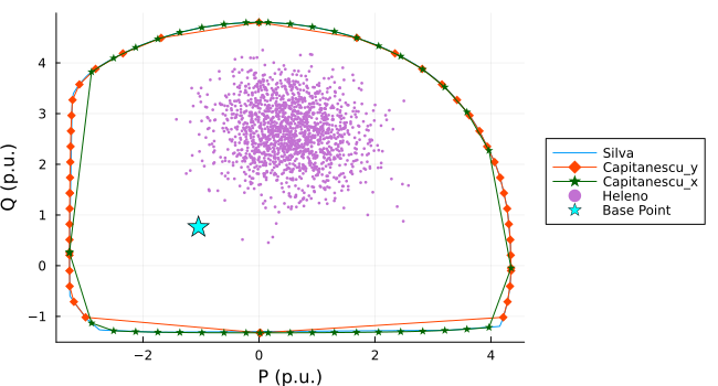
[4], [5] propose an OPF-based method to estimate the flexibility region. The method involves solving a series of OPF problems to find the maximum and minimum active and reactive power that can be injected or absorbed at the TSO-DSO interface while satisfying all network constraints.
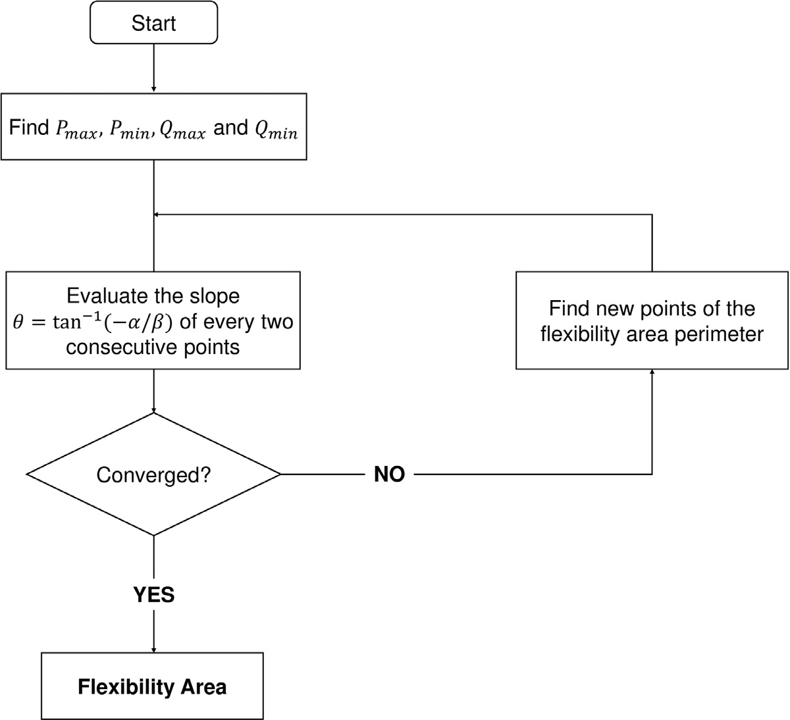
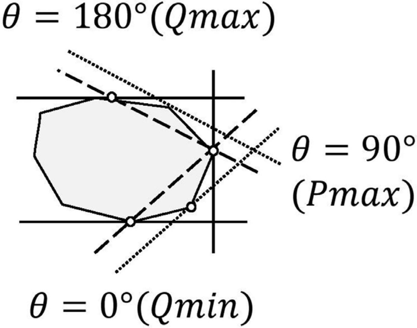
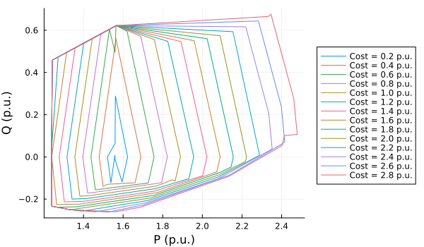
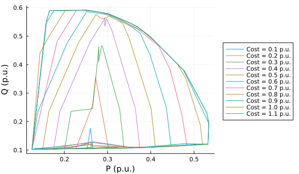
[5] also proposed a method to estimate the cost of the flexibility by adding a cost constraint in the OPF problem. The cost constraint is gradually increased until the flexibility region no longer expands.
Pros:
- captures the network constraints
- gives larger flexibility region than the Monte Carlo envelope method
- easy to scale to larger networks
Cons:
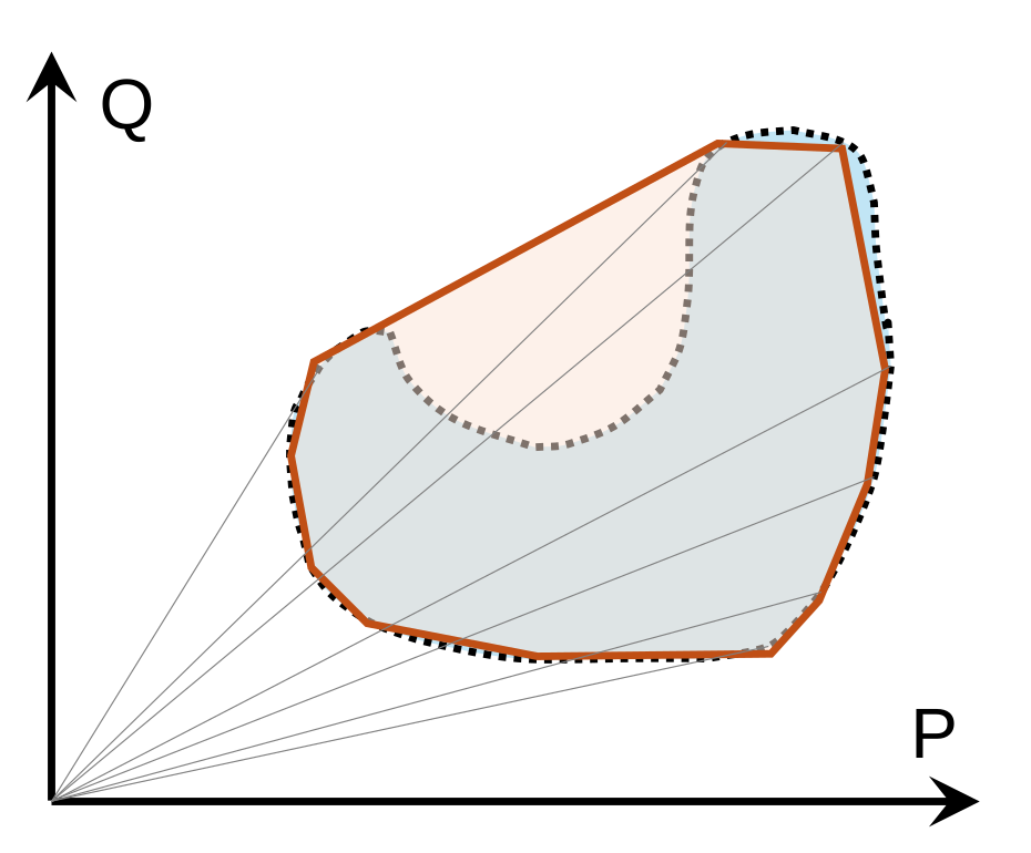
- the grid constraints are not guaranteed to be satisfied within the estimated hull due to the non-convexity, see Figure 4.
Fixed Direction Search Method
[6] proposed a similar method to estimate the flexibility region. Instead of using tangent lines, the search directions are fixed to the coordinate axes. In the original paper:
- solve 4 OPF problems to find the maximum and minimum active and reactive powers: \(P_\text{min}\), \(Q_\text{min}\), \(P_\text{max}\), \(Q_\text{max}\);
- along the \(Q\) axis, add constraints \(Q\geq Q_\text{min} + m\cdot\Delta Q\), and solve for the maximum and minimum \(P\) to get the points on the upper and lower boundaries until \(Q_\text{max}\) is reached;
- make an envelope of the points to get the flexibility region.
Similar to the tangent line search method, this method implied a convexity assumption of the flexibility region, which is not always true.
Instead of using inequality constraints to search along the \(Q\) axis, we can use equality constraints to directly search for the points on the shape boundary, which can capture the non-convexity of the flexibility region to some extent.
Moreover, the search directions are also extended to the \(P\) axis, which can further capture the non-convexity of the flexibility region. The search procedure is illustrated in Figure 5.
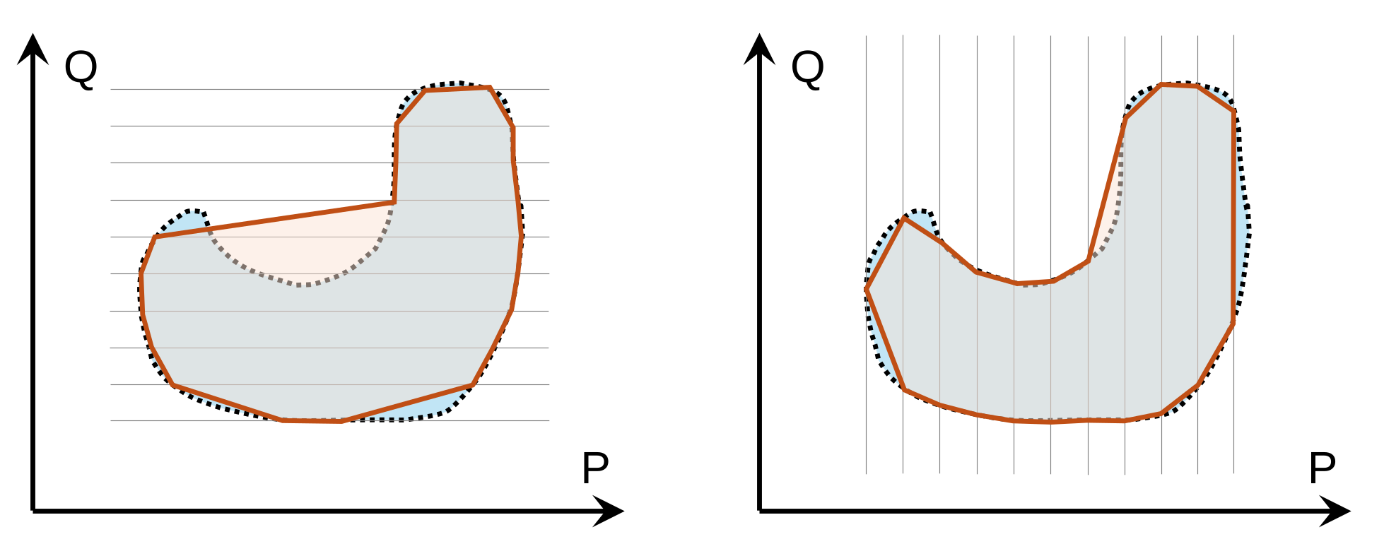
However, the non-convexity of the flexibility region is still not fully captured, another thing issued is that how to apply the non-convex flexibility region in the TSO-DSO coordination.
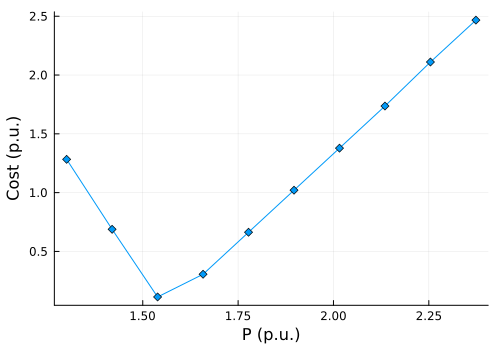
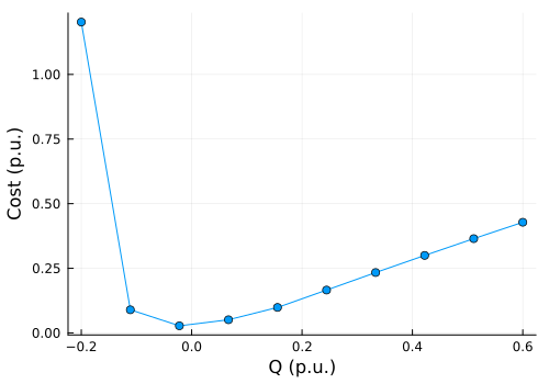
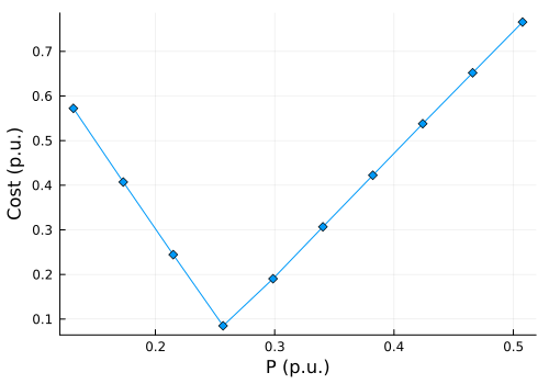
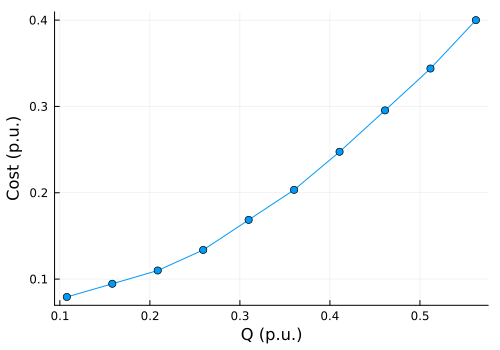
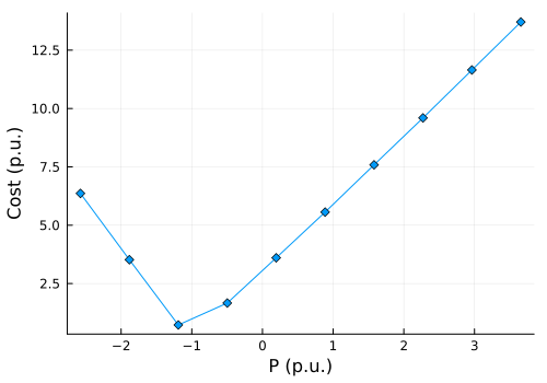
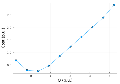
[7] further proposed a method to estimate the cost curves of active and reactive power flexibility by decoupling the cost minimization along the \(P\) and \(Q\) axes. The process:
- solve 4 OPF problems to find the maximum and minimum active and reactive powers: \(P_\text{min}\), \(Q_\text{min}\), \(P_\text{max}\), \(Q_\text{max}\);
- along the \(P\) axis, add constraints \(P = P_\text{min} + m\cdot\Delta P\), and solve for the minimum cost to get the cost curve of active power flexibility until \(P_\text{max}\) is reached;
- along the \(Q\) axis, add constraints \(Q = Q_\text{min} + m\cdot\Delta Q\), and solve for the minimum cost to get the cost curve of reactive power flexibility until \(Q_\text{max}\) is reached;
- two decoupled cost curves are given.
Implementation of Static Methods
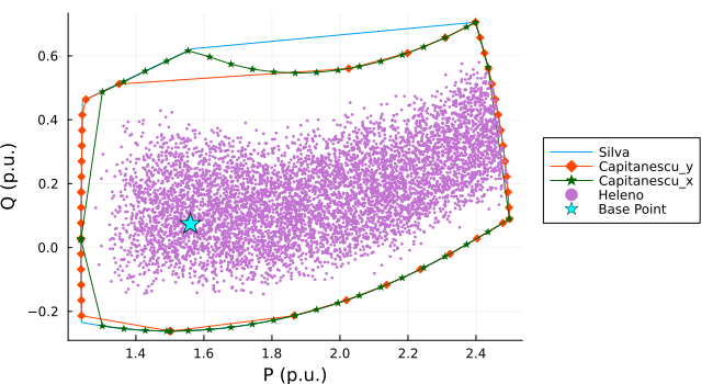
IEEE 9-bus System
System configuration:
- 2 generators: 1 RES and 1 synchronous compensation
- 3 flexible loads that can be curtailed by up to 10%
IEEE 33-bus System
System configuration:
- 8 curtailable RES generators
- 2 battery storage systems that could work in 4 quadrants
118-bus System
System configuration from [8] with modifications:
- 11 curtailable RES generators
- 5 battery storage systems that could work in 4 quadrants
- 5 flexible loads that can be curtailed by up to 10%
Let the feasible set of all complex power injections in the ACOPF problem be denoted as \[ \mathcal{S}_{\text{feas}} \subset \mathbb{C}^N \]
The slack bus power \(s_0 = p_0 + j q_0\) is simply one component of the full injection vector \(s\). Extracting \(s_0\) from \(s\) is equivalent to applying a projection operator \(\Pi_0\) onto the 0-th coordinate: \[ s_0 = \Pi_0(s) \]
The operator \(\Pi_0\) is a purely linear mapping from \(\mathbb{C}^N \to \mathbb{C}\).
Theorem: the image of a convex set under a linear transformation is strictly convex.
Therefore, if the global solution space of injections \(\mathcal{S}_{\text{feas}}\) is convex, its projection onto the \(P_0-Q_0\) plane must inherently be a convex set.
The problem becomes: find the conditions under which \(\mathcal{S}_{\text{feas}}\) is convex.
Equivalently, the solvability set of a power network, i.e., the set of all power injection vectors for which the corresponding power flow equations admit a solution, need to be convex.
[9] shows that the solvability set of a power network without grid operational constraints, is convex:
- For networks with a radial topology if and only if the network is homogeneous. A homogeneous network is one where all lines share the exact same \(r/x\) ratio.
- If the analysis is restricted solely to active power injections, the solvability set is convex for any connected network with a radial topology, regardless of homogeneity.
- The active power solvability set is also convex for purely resistive networks of any arbitrary topology (including meshed grids).
[10] gives a convex restriction for the ACOPF feasibility set (solution space with operational constraints), which is a convex inner approximation of the true feasibility set, shown in Figure 14.
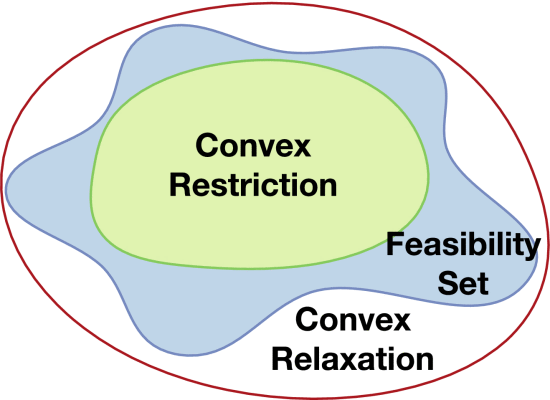
The original non-convex feasibility set defined by the AC power flow equations and operational constraints: \[ \begin{align*} p_i^\text {inj}&=\sum _{k\in \mathcal {N}} v_iv_k(G_{ik}\cos \theta _{ik}+B_{ik}\sin \theta _{ik}) \quad i\in \mathcal {N} \\ q_i^\text {inj}&=\sum _{k\in \mathcal {N}} v_iv_k(G_{ik}\sin \theta _{ik}-B_{ik}\cos \theta _{ik}) \quad i\in \mathcal {N} \\ q_i^\text {min}&\leq q_i^\text {inj}\leq q_i^\text {max} \quad i\in \mathcal {N}_G \\ v_i^\text {min}&\leq v_i\leq v_i^\text {max} \quad i\in \mathcal {N}_\text {pq} \\ \varphi ^\text {min}_l&\leq \theta _l^\text {f}-\theta _l^\text {t}\leq \varphi ^\text {max}_l \quad l\in \mathcal {E} \end{align*} \] is restricted to the following QP convex restriction: \[ \begin{aligned} K^+\overline{g}_\mathcal {P}+K^-\underline{g}_\mathcal {P}&\leq b \\ L^+\overline{\psi }_\mathcal {P}+L^-\underline{\psi }_\mathcal {P}&\leq d, \quad b\leq b^{\text{max}} \\ \end{aligned} \] where: \[ \begin{aligned} b&=\begin{bmatrix}\overline{\varphi }^T &\quad \overline{v}^T_\text {pq} &\quad -\underline{\varphi }^T &\quad -\underline{v}^T_\text {pq} \end{bmatrix}^T \\ \overline{g}_\mathcal {P}&=\begin{bmatrix}p_\text {ns}^T &\quad q_\text {pq}^T &\quad {\overline{g}^C_\mathcal {P}}^T &\quad {\overline{g}^S_\mathcal {P}}^T &\quad {\overline{g}^Q_\mathcal {P}}^T \end{bmatrix}^T \\ \underline{g}_\mathcal {P}&=\begin{bmatrix}p_\text {ns}^T &\quad q_\text {pq}^T &\quad {\underline{g}^C_\mathcal {P}}^T &\quad {\underline{g}^S_\mathcal {P}}^T &\quad {\underline{g}^Q_\mathcal {P}}^T \end{bmatrix}^T \\ \overline{\psi }_\mathcal {P}&=\begin{bmatrix}p_\text {ns}^T &\quad q_\text {pq}^T &\quad {\overline{\psi }^C_\mathcal {P}}^T &\quad {\overline{\psi }^S_\mathcal {P}}^T &\quad {\overline{\psi }^Q_\mathcal {P}}^T \end{bmatrix}^T \\ \underline{\psi }_\mathcal {P}&=\begin{bmatrix}p_\text {ns}^T &\quad q_\text {pq}^T &\quad {\underline{\psi }^C_\mathcal {P}}^T &\quad {\underline{\psi }^S_\mathcal {P}}^T &\quad {\underline{\psi }^Q_\mathcal {P}}^T \end{bmatrix}^T. \end{aligned} \]
in which \[ g(x,u)= \begin{bmatrix}p^\text {inj}_\text {ns} \\ q^\text {inj}_\text {pq} \\ v^\text {f} v^\text {t}\cos \tilde{\varphi }-v^\text {f}_0v^\text {t}-v^\text {f}v^\text {t}_0 \\ v^\text {f} v^\text {t}\sin \tilde{\varphi }-v^\text {f}_0v^\text {t}_0\varphi \\ v^2-2v_0v \end{bmatrix} \]
and variables \(g_\mathcal {P}^C\), \(g_\mathcal {P}^S\), \(g_\mathcal {P}^Q\) with overlines and underlines denote the variables representing the interval bounds of the non-linear elements (cosine, sine and quadratic) over the self-mapping set.
The method from [10] cannot be used to get a convex approximation of the flexibility region:
- cannot add the slack bus active power (\(p_{\text{slack}}^{\text{inj}}\)) to the control vector \(u\), since \(u\) represents a set of strictly independent variables.
- The slack bus must remain a dependent variable that absorbs the mismatch and state-dependent losses to guarantee solvability.
That means the convex restriction can only be applied to the non-slack injection space, but not to the projected \(P_0-Q_0\) space, which is the flexibility region we are interested in.
Time-coupled Methods
Hyperbox Approximation
[11] focused the total potential energy flexibility (in MWh) without considering the reactive power flexibility.
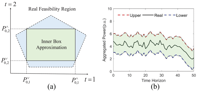
Define the flexibility region as a hyperbox \(\mathbb{S}\): \[ \mathbb {S}=\left [{{P}^\vee _{\text{td},1}, {P}^\wedge _{\text{td},1}}\right]\times \left [{{P}^\vee _{\text{td},2}, {P}^\wedge _{\text{td},2}}\right]\times {\dots } \times \left [{{P}^\vee _{\text{td},T}, {P}^\wedge _{\text{td},T}}\right] \]
Objective: maximize the total aggregated energy flexibility over the time horizon \(T\): \[ \max E_{af} \mathrel {\mathrel {\mathop :}=}\sum _{t\in \mathcal {T}} \left ({{P}^\wedge _{\text{td},t}-{P}^\vee _{\text{td},t} }\right)\cdot \Delta t \]
Constraints:
- power flow: fixed-point single-step approximation method from [3], claiming a better performance than the first order Taylor expansion method; \[ \tilde { \mathbf {v}}= \mathbf {M} \mathbf {x} + \mathbf {m} \] \[ \tilde { \mathbf {s}}_0= \mathbf {G} \mathbf {x} + \mathbf {g} \]
- voltage limits: between 0.9 p.u. to 1.1 p.u.;
- device constraints;
- joint sanity constraints: \[ {P}^\wedge _{\text{td},t} \geq {P}^\vee _{\text{td},t}\quad \forall t\in \mathcal {T} \]
Pros:
- computationally very efficient
- decouple the time dimension, allowing for easier analysis of temporal flexibility
Cons:
- a very conservative inner approximation of the flexibility region
- the fixed-point linear power flow approximation may not be accurate globally for large flexibility regions
- does not capture the uncertainties
Decouple P and Q
[12] and [13] decouple the active and reactive power flexibility and find the upward and downward flexibility separately. The method is still a conservative hyperbox approximation with introducing a TSO priority weight \(w_{t}^\text{TSO}\) to the objective function to capture the TSO’s preference on the flexibility at different time steps.
Objective: maximize the weighted sum of the active and reactive power flexibility over the time horizon \(T\): \[ \begin{align*} \lbrace {\underline{P}}_{t}^\text{td} | t \in {\mathcal T}\rbrace = & \arg \min \sum _{t \in {\mathcal T}} w_{t}^\text{TSO} P_{t}^\text{td} \\ \lbrace {\overline{P}}_{t}^\text{td} | t \in {\mathcal T}\rbrace = & \arg \max \sum _{t \in {\mathcal T}} w_{t}^\text{TSO} P_{t}^\text{td} \\ \lbrace {\underline{Q}}_{t}^\text{td} | t \in {\mathcal T}\rbrace = & \arg \min \sum _{t \in {\mathcal T}} w_{t}^\text{TSO} Q_{t}^\text{td} \\ \lbrace {\overline{Q}}_{t}^\text{td} | t \in {\mathcal T}\rbrace = & \arg \max \sum _{t \in {\mathcal T}} w_{t}^\text{TSO} Q_{t}^\text{td} \end{align*} \]
Constraints:
- power flow: non-linear AC power flow equations
- voltage limits: between 0.9 p.u. to 1.1 p.u.;
- device constraints;
- joint sanity constraints: \[ \begin{align*} P_{t}^\text{td} \geq P_{t}^\text{td, plan} \quad \forall t\in \mathcal {T} \\ P_{t}^\text{td} \leq P_{t}^\text{td, plan} \quad \forall t\in \mathcal {T} \end{align*} \]
Pros:
- computationally efficient
- allows for capturing the TSO’s preference on the flexibility at different time steps
Cons:
- still conservative
- does not capture the uncertainties
Ellipsoid Approximation
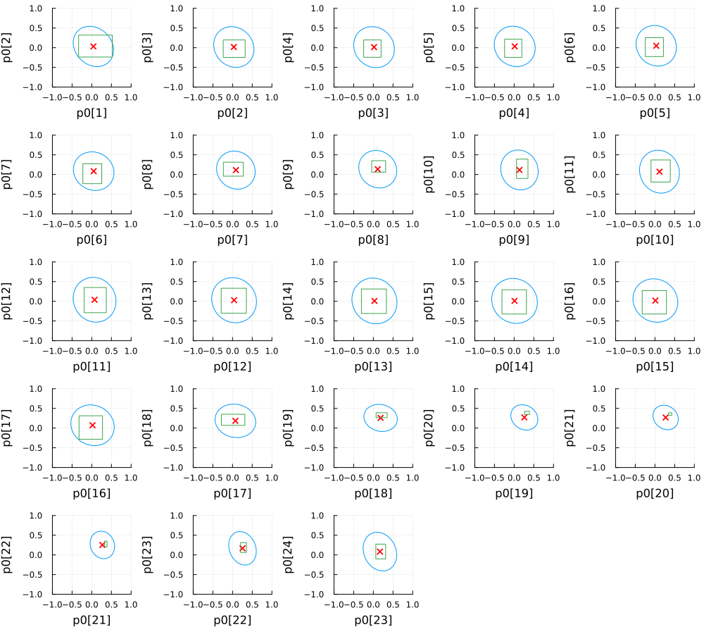
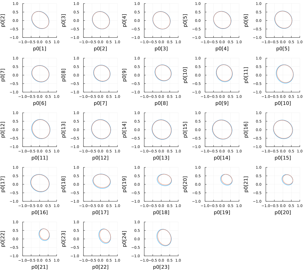
[14] formulate the flexibility region estimation as an adaptive robust optimization problem which is to maximize the volume of an ellipsoid (MVE) inscribed in the true flexibility region. The method is less conservative than the hyperbox approximation.
Objective: maximize the volume of the inscribed ellipsoid, which is equivalent to maximizing \(\log\det \mathbf{E}\).
Constraints:
- power flow: fixed-point single-step approximation method from [3], claiming a better performance than the first order Taylor expansion method; \[ \tilde { \mathbf {v}}= \mathbf {M} \mathbf {x} + \mathbf {m} \] \[ \tilde { \mathbf {p}}_0= \mathbf {G} \mathbf {x} + \mathbf {c} \]
- voltage limits: between 0.9 p.u. to 1.1 p.u.;
- device constraints with load uncertainties modeled by \(\boldsymbol{\zeta}\) where \(\Vert \boldsymbol{\zeta}_{t}\Vert\leq 1\);
The constraints are written in compact form as: \[ \mathbf{Dp} +\mathbf{b}(\boldsymbol{\zeta}) = {\mathbf {p}}_0 \quad \mathbf{Wp} \leq \mathbf{z}(\boldsymbol{\zeta}) \]
The final optimization problem is: \[ \begin{align*} \max_{\mathbf{e},\mathbf{E}\succeq 0}& \ \log\det \mathbf{E} \\ & \forall \ \Vert \boldsymbol{\xi} \Vert\leq 1,\forall\Vert \boldsymbol{\zeta}_{t}\Vert\leq 1\\ & t=1, \ldots, T \\ & \exists \ \mathbf{p} \\ \mathrm{s.t.} & \ \mathbf{E}\boldsymbol{\xi}+\mathbf{e}= \mathbf{Dp} +\mathbf{b}(\boldsymbol{\zeta})\\ & \ \mathbf{Wp} \leq \mathbf{z}(\boldsymbol{\zeta}) \end{align*} \] which is reformulated as a tractable convex approximation below (SOCP) via the affine policy: \[ \begin{align*} &\max\limits_{\mathbf{E}\succeq 0,\mathbf{e},\mathbf{K},\{\mathbf{L}_{t}\}_{t=1}^{T},\boldsymbol{\gamma},\{\alpha_{i}\}_{i=1}^{m}}\log \det\mathbf{E}\\ &\ \ \mathrm{s.t}.\qquad (\forall i=1, \ldots, m)\\ &\Vert \mathbf{w}_{1,i}\tilde{D}^{-1}\mathbf{E}+\mathbf{w}_{2,i}\mathbf{K}\Vert+ \sum\limits_{k=1}^{T}\Vert \mathbf{w}_{2,i}\mathbf{L}_{k}- \boldsymbol{\theta}_{k, i}\Vert\leq \alpha_{i},\\ &\alpha_{i}+\mathbf{w}_{1,i}\tilde{\mathbf{D}}^{-1}\mathbf{e}+\mathbf{w}_{2,i}\boldsymbol{\gamma}- \nu_{i}\leq 0, \end{align*} \]
Pros:
- less conservative than the hyperbox approximation
- captures the uncertainties in the load
Cons:
- computationally more intensive than the hyperbox approximation
- the fixed-point linear power flow approximation may not be accurate globally for large flexibility regions
- does not capture the uncertainties of the DERs
Implementation of Time-coupled Methods
IEEE 33-bus System
Aggregated P Flexibility
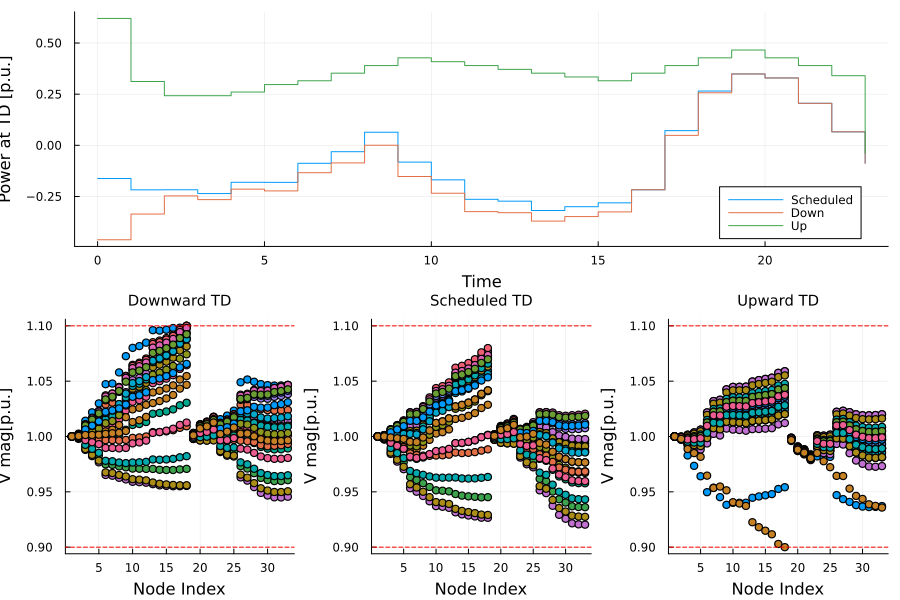
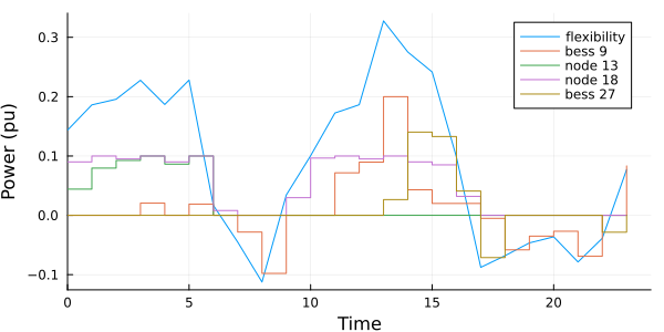
The active power flexibility at the TSO-DSO interface is disaggregated to the flexible devices via solving an optimization problem with the objective of minimizing the total cost of the operation point deviation from the original plan, subject to the power flow constraints and device constraints.
Hyperbox vs Ellipsoid Approximation
Future Work
- Convex approximation of the non-convex flexibility region, while the discontinuity of the flexibility region is a challenge.
- Application of the flexibility region for TSO-DSO coordination
- at the TSO side, how to efficiently use the flexibility region reported by the DSOs?
- at the DSO side, how to efficiently disaggregate the flexibility request from the TSO to the flexible devices?
- How to identify the convexity of the flexibility region under certain conditions? If the region is non-convex, how “close” the convex hull is to the true flexibility region?
- Introduce uncertainties
- Contingency analysis