The convex approximation of Flexibility Regions at TSO-DSO Interfaces with SOCP Relaxation

Problem Statement
\[ \mathcal{R} = \{(P_0, Q_0) \in \mathbb{R}^2 : \text{power flow equation, and operational constraints}\} \]
The boundary scanning method from [1] allows us to approximate the flexibility region from the outside by solving a series of OPF problems.
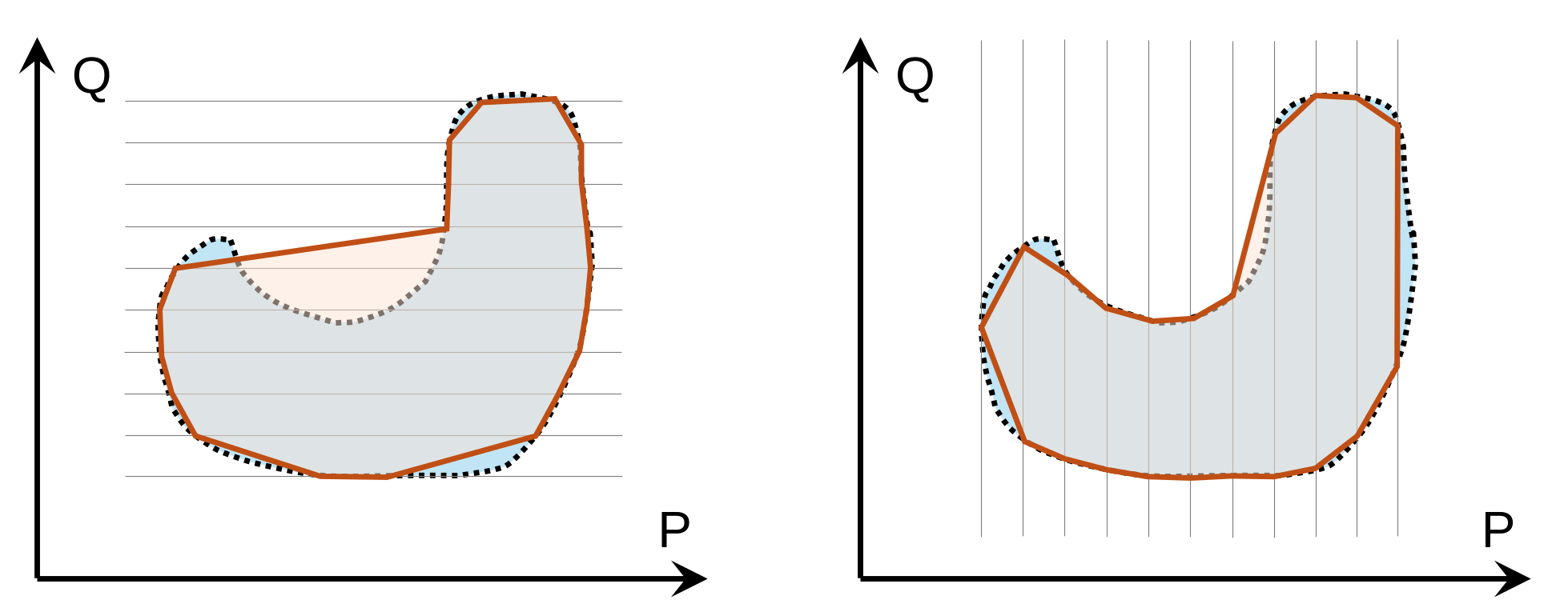
However, the flexibility region is not convex in general. Without guarantees of convexity, it is difficult to use the flexibility region and derive cost functions.
A Case Study of the Convexity
IEEE 33-bus System
System configuration:
- 8 curtailable RES generators
- 2 battery storage systems that could work in 4 quadrants
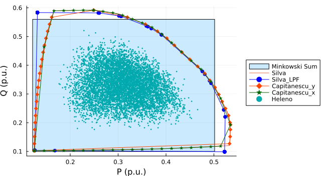
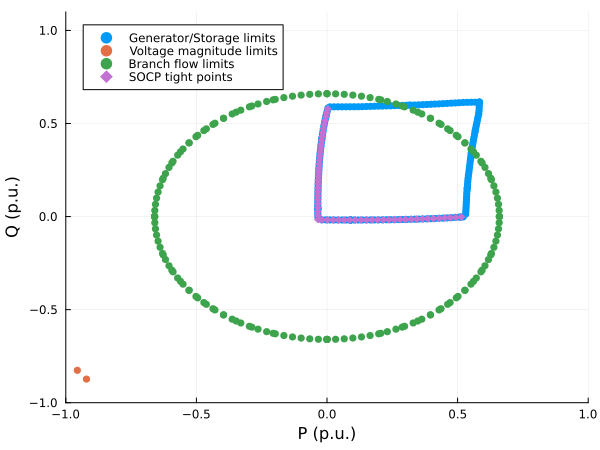
The left and bottom edges of the flexibility region are convex.
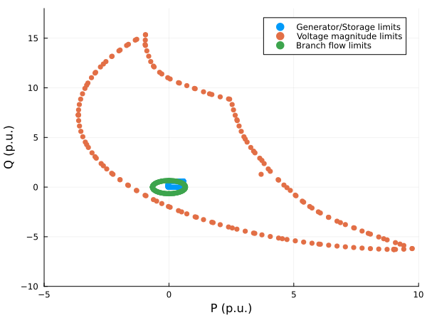
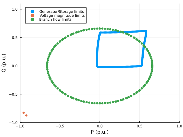
Convexity of the left and bottom edges of the flexibility region with the injection limits
Let:
- \(x\) the active power injection at the slack bus
- \(y\) the reactive power injection at the slack bus
- \(\lambda\) the vector of all other injection variables, \(\Lambda\) a convex feasible set of \(\lambda\)
- \(F(x,y,\lambda) = 0\) the AC power flow equations (non-convex)
The bottom boundary is given by minimizing \(y\) for a given \(x\): \[ f(x) = \inf_{y, \lambda} \{ y \mid (x, y, \lambda) \in \mathcal{S} \} \] where \(\mathcal{S} = \{ (x, y, \lambda) \mid F(x,y,\lambda) = 0, \lambda \in \Lambda \}\) and the flexibility region is given by \(\mathcal{R} = \{ (x,y) \mid \exists \lambda: (x, y, \lambda) \in \mathcal{S} \}\).
The left boundary is given by minimizing \(x\) for a given \(y\): \[ g(y) = \inf_{x, \lambda} \{ x \mid (x, y, \lambda) \in \mathcal{S} \} \]
Because the objective function is linear and therefore convex, \(f(x)\) and \(g(y)\) will be convex if the set \(\mathcal{S}\) is convex.
With SOCP relaxation: \[ f_\text{relaxed}(x) = \min_{y, \lambda} \{ y \mid F_\text{relaxed}(x,y,\lambda) \le 0, \lambda \in \Lambda \} \] Then \(F_\text{relaxed}\) represents a convex set (the intersection of affine hyperplanes and second-order cones), \(f_\text{relaxed}(x)\) and \(g_\text{relaxed}(y)\) are convex functions.
If the SOCP relaxation is exact for every boundary point, then \(F_\text{relaxed}(x,y,\lambda) \le 0\) is equivalent to \(F(x,y,\lambda) = 0\), and the convexity of \(f(x)\) and \(g(y)\) is ensured.
\(g(x)\) and \(f(y)\), i.e., the left and bottom envelopes of the flexibility region with the injection limits, are convex functions if the SOCP relaxation of the AC power flow equations is exact along the boundaries.
AC Power Flow Problems in the Lifted Space
From [2], we learn that the AC power flow equations can be reformulated in a lifted space \(\Psi\).
Starting from the radial AC network, define the lifted variables collected into \(\Psi\):
\[ w_i = |V_i|^2, \]
\[ c_{ik} = V_iV_k\cos(\theta_i-\theta_k), \]
\[ s_{ik} = V_iV_k\sin(\theta_i-\theta_k). \]
The flexibility outputs are linear functions of the lifted variables:
\[ y= \begin{bmatrix} P_s\\ Q_s \end{bmatrix} = C_s\Psi. \]
Let \(u\) represent injections at non-slack buses, all operational quantities become linear:
\[ u=C_{ns}\Psi. \] with injection limits: \[ Au\le b. \]
Operational constraints (voltage limits and line flow limits) are represented as
\[ M\Psi\le m. \]
The only remaining non-convexity is just the rank-1 condition for the \(\Psi\) space:
\[ c_{ik}^2+s_{ik}^2=w_iw_k. \]
Thus the AC flexibility problem becomes
\[ \begin{aligned} &y = C_s\Psi,\\ &u = C_{ns}\Psi,\\ &Au \le b,\\ &M\Psi \le m,\\ &c_{ik}^2+s_{ik}^2 = w_iw_k. \end{aligned} \]
The goal is to characterize a larger region of \(y \in \mathbb{R}^2\).
Suppose we have a sufficient condition guaranteeing existence and uniqueness (e.g., [3]) for every feasible \(u\) \[ \Psi = \phi(u), \] where \(\phi\) is a nonlinear, implicit function. Then we can write \[ y = C_s\phi(u) =: G(u), \] where \(G\) is a nonlinear transfer function from the non-slack bus injections to the slack bus injections.
Try to eliminate \(\Psi\): \[ \Psi = \Psi_0 + N \alpha + R u \] where \(\Psi_0\) is a base operation point, \(N\) is a basis for the null space of the linear constraints, and \(R\) is a particular solution.
Then \[ y = C_s(\Psi_0 + N \alpha + R u) \]
All nonlinearity is now pushed into the feasible set of \(\alpha: \mathbb{R}^{2n-2} \rightarrow \mathbb{R}^2\), the term \(C_s N \alpha\) actually represents the nonlinear active and reactive power losses.
One may then try to construct an explicit approximation of the \(\alpha\) function, e.g., Taylor expansion …
However, the tracking of the operational constraints is lost (defined explicitly in the space of \(\Psi\)) …
SOCP Approximation of the Flexibility Region in the Lifted Space
SOCP Relaxation
Replace
\[ c_{ik}^2+s_{ik}^2=w_iw_k \]
with
\[ c_{ik}^2+s_{ik}^2\le w_iw_k. \]
For radial networks this corresponds to relaxing the rank-1 condition of the AC power flow equations.
The feasible set becomes convex:
\[ \mathcal X \subseteq \mathcal X_{\rm soc}. \]
Its projection onto
\[ (P_s,Q_s) \]
is therefore also convex.
Explicit Losses-aware Flexibility Region
The key observation is that the problematic portions of the flexibility boundary are associated with inefficient operating points that trying to maximize losses (the right and top boundaries we observe in Figure 2).
Since total losses are also linear in the lifted variables,
\[ P_{\rm loss} = l_P^T\Psi \sum_{(i,k)} = g_{ik} (w_i+w_k-2c_{ik}), \]
an explicit losses budget can be imposed:
\[ P_{\rm loss}\le \eta_p \quad Q_{\rm loss}\le \eta_q \]
\(\eta_p\) and \(\eta_q\) can be calculated using NLP-based methods (solving 2 OPF problems to estimate).
The resulting feasible set is
\[ \mathcal X_{\rm soc,\eta} \subseteq \mathcal X_{\rm soc}. \]
This step intentionally sacrifices a small amount of flexibility in exchange for:
- avoidance of inefficient operating points,
- improve relaxation tightness,
- preservation of convexity.
If the exactness of the SOCP relaxation is guaranteed for all boundary points, then \(\mathcal X_{\rm soc,\eta}\) is an inner convex approximation of the original flexibility region \(\mathcal X\).
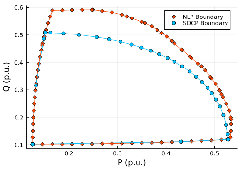
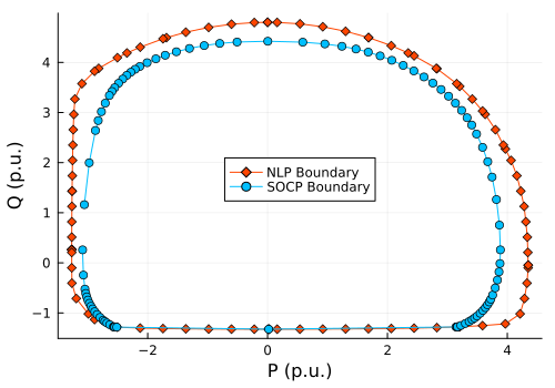
- We cannot guarantee that the SOCP relaxation is exact for all points on the boundary.
- The maximization problem will lead to a maximization of losses, which gives a huge relaxation gap.
- We assume that, with a small losses budget, the relaxation gap will be small / acceptable and only lead to a small neighborhood of the feasible states. (Need to be investigated further)
- We could check the exactness numerically as a post-processing step by solving the original AC power flow equations for the boundary points.
Define the lifted-space relaxation gap
\[ \delta_{ik} = w_iw_k-c_{ik}^2-s_{ik}^2. \]
Using the equivalence with DistFlow variables,
\[ \Delta_{ik} = w_i l_{ik} = (P_{ik}^2+Q_{ik}^2) = |y_{ik}|^2\delta_{ik}. \]
The branch losses can be decomposed as: \[ P_{ik}^{loss} = r_{ik} \frac{P_{ik}^2+Q_{ik}^2}{w_i} + \frac{r_{ik}|y_{ik}|^2}{w_i} \delta_{ik}. \]
Therefore: \[ P_{ik}^{loss} - P_{ik,phys}^{loss} = \frac{r_{ik}|y_{ik}|^2}{w_i} \delta_{ik}. \]
This establishes that relaxation gap is exactly proportional to excess losses beyond the physically realizable losses.
The bounds can be derived for:
Current error
\[ |l_{ik}-\hat l_{ik}| = \frac{|y_{ik}|^2}{w_i}\delta_{ik}. \]
Voltage error
\[ |v_i^{soc}-v_i^{ac}| \le C_V \sum_{(i,k)\in E} \delta_{ik}. \]
Instead of proving exact AC feasibility, we quantify the distance to an AC-feasible solution.
Because \(\mathcal X_{\rm soc,\eta}\) is convex, its projection \(\mathcal F_{\rm soc,\eta} = \{y=C_s\Psi\}\) is also convex.
Unlike the traditional boundary tracing, the flexibility region can therefore be represented by:
- the SOCP model itself as a convex constraint,
- explicit polyhedral approximations (e.g. boundary points → convex hull, supporting hyperplanes),
- inner ellipsoids,
- …
Flexibility cost
Introduce a convex operating cost \(J(\Psi)\), define the value function:
\[ f(P_s,Q_s) = \min_{\Psi} J(\Psi) \]
Since the feasible set is convex, with a convex cost function, the dual multipliers associated with
\[ P_s=P_s^{target}, \qquad Q_s=Q_s^{target} \]
satisfy
\[ \nabla f(P_s,Q_s) = \begin{bmatrix} \lambda_P\\ \lambda_Q \end{bmatrix}. \]
The dual multipliers can be interpreted as the marginal cost.
Numerical Examples
| Case | Time NLP [s] | Memory NLP [MB] | Time SOCP [s] | Memory SOCP [MB] | Area Ratio |
|---|---|---|---|---|---|
| 12-node | 0.11 | 34.8 | 0.08 | 12.1 | 0.60 |
| 33-node | 0.20 | 102.2 | 0.16 | 42.3 | 0.82 |
| 69-node | 0.44 | 243.7 | 0.43 | 115.9 | 0.84 |
| 74-node | 0.56 | 268.1 | 0.57 | 127.7 | 0.38 |
| 85-node | 0.51 | 312.2 | 0.56 | 160.0 | 0.71 |
| 94-node | 0.69 | 358.6 | 0.71 | 191.2 | 0.54 |
| 118-node | 0.87 | 488.4 | 0.77 | 274.3 | 0.98 |
Current Challenges
SOCP Exactness
To get an explicit expression for the flexibility region, the boundary is obtained by solving a sequence of support-function maximization problems:
\[ \max d^T y \]
The existing exactness guarantees for radial OPF (AROPF [4]) no longer apply because the objective is not monotonically increasing at the slack bus.
The current approach relies on post-processing verification of the relaxation gap, which is not theoretically strict.
Meshed networks are even more challenging …
Selection of the Losses Budget
The explicit losses budget
\[ P_{\rm loss}\le \eta_p \qquad Q_{\rm loss}\le \eta_q \]
- A small value improves the tightness of the SOCP relaxation, but sacrifices flexibility.
- A large value increases the flexibility region, but may lead to a large relaxation gap.
Current approach first solves 2 NLP OPF problems to estimate:
\[ \eta_p: \max (+P_s - Q_s) \qquad \eta_q: \max (- P_s + Q_s) \]
If the relaxation gap is too large, the losses budget is gradually reduced until the relaxation gap is acceptable. This is a heuristic approach and may not be optimal.
Numerical instability
Some test cases (e.g., 74-node) returns numerically unstable status when trying to maximize the consumption at the slack bus.
Current approach drops the problematic boundary points and uses the remaining points, which creates a cut and loses some flexibility.
For radial networks, we know that the SDP and SOCP relaxations are theoretically equivalent.
We observe that the SDP relaxation is more numerically stable than the SOCP relaxation (for the same case, the SDP relaxation successfully computes numerically difficult points for the SOCP relaxation). However, the SDP relaxation is much more computationally expensive (~10x slower).
Flexibility cost function
The value function provides a natural definition of the optimal flexibility cost: \[ f(P_s,Q_s) = \min_{\Psi} J(\Psi) \]
Currently, the cost function is defined by point-wise evaluation of the value function within the estimated flexibility region.