An Explicit Convex Inner Approximation of AC Power Flexibility at the TSO–DSO Interface in Radial Networks

Introduction
The flexibility region (FR) is a set of feasible active and reactive power injections at the TSO-DSO interface, which is defined by the AC power flow equations and operational constraints. The FR is a fundamental concept for TSO-DSO coordination, as it provides a compact representation of the DSO’s capabilities to support the transmission system while keeping the privacy of the DSO.
Recent studies have proposed various methods to estimate the FR, including Monte-Carlo searching [1] and boundary scanning methods [2], [3]. However, [4] has indicated that the FR is generally non-convex, and the boundary scanning methods may result in non-convex “Polygonal” FRs, which are not only unsuitable for optimization and control applications, but also may lead to infeasible operating points close to the boundary.
The goal of this work is to provide an explicit, convex, inner approximation of the FR in radial networks using a losses-regularized augmented relaxed optimal power flow (AROPF) formulation proposed in [5]. The proposed method leverages the SOCP relaxation of the AC power flow equations with considering the transverse parameters, a set of more conservative constraints are imposed to restrict feasible set and ensure the exactness of the SOCP relaxation.
The proposed method is validated on several radial distribution networks, and the results show that the proposed method can provide a reliable convex inner approximation of the FR with efficient computational performance and low conservatism. Using the proposed method, the FR can be represented as a polygon, which can be efficiently used for optimization and control applications.
Problem Statement
\[ \mathcal{R} = \{(P_0, Q_0) \in \mathbb{R}^2 : \text{power flow equation, and operational constraints}\} \]
The boundary scanning method from [2], [3] allows us to approximate the flexibility region from the outside by solving a series of OPF problems.
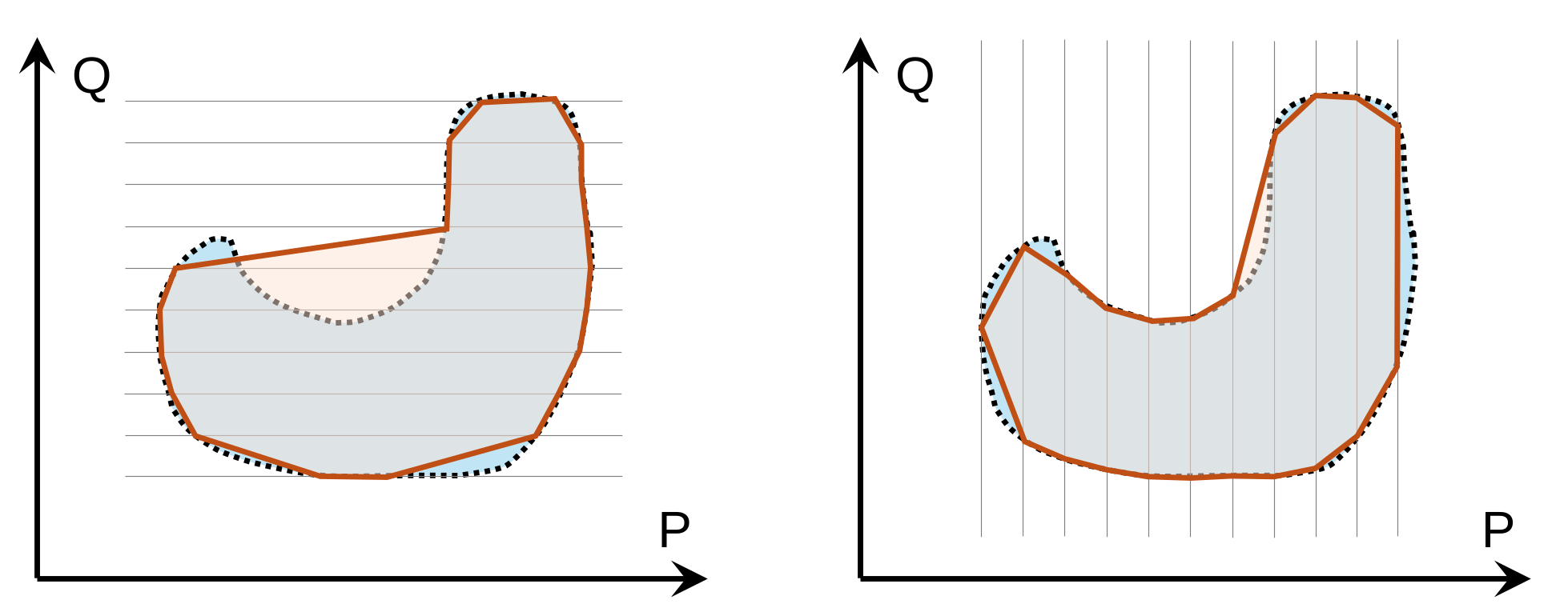
However, the flexibility region is not convex in general. Without guarantees of convexity, it is difficult to use the flexibility region and derive cost functions.
Our Goal: Explicit, Convex, Inner
Existing approaches often sacrifice at least one of these. For example, AC-OPF boundary tracing can retain AC fidelity but is nonlinear thus loses the convexity. Linear/polyhedral approaches are attractive computationally but rely on approximations of the AC network. There is existing work specifically on convex and explicit approximations of aggregate flexibility, but much of it is built around linearized distribution models and therefore not exact (not inner approximations).
Methodology
From [5], we learn the AROPF can provide an exact convex representation of the AC power flow equations in radial networks. The AROPF formulation is based on the SOCP relaxation of the AC power flow equations, which is known to be exact for radial networks under certain sufficient conditions. The AROPF formulation introduces a set of auxiliary variables and constraints to augment the feasible set and ensure the exactness of the SOCP relaxation.
Write the AROPF in a compact form: \[ \begin{aligned} \min & \quad J(\Psi) \\ \text{s.t. } & \quad \Psi \in \mathcal{X}_{\rm AROPF} \end{aligned} \] where \(\Psi\) is the set of variables (e.g., nodal injections and voltages), \(\mathcal{X}\) represents the feasible solution set defined by the non-linear AC power flow equations and operational constraints, and \(\mathcal{X}_{\rm AROPF}\) is the feasible solution set defined by the SOCP relaxation of the AC power flow equations, the operational constraints, and the augmented constraints. By defining a set of convex operational constraints, the \(\mathcal{X}_{\rm AROPF}\) is convex. Moreover, we have \(\mathcal{X}_{\rm AROPF} \subseteq \mathcal{X}\) if the sufficient conditions for exactness are met, shown in Figure 2.
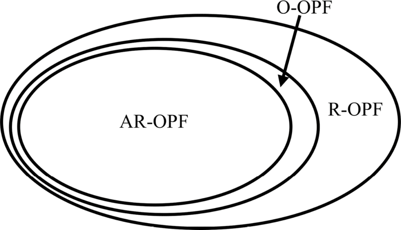
Denote the flexibility (the active and reactive power at the slack bus) as \(y = C_s\Psi\in \mathcal{Y}\), \(\mathcal{Y}\) is the projection (\(C_s\)) of the feasible set \(\mathcal{X}\) onto the \((P_s, Q_s)\) space. Due to the non-convexity of the AC power flow equations, \(\mathcal{X}\) and its projection \(\mathcal{Y}\) are non-convex in general.
- Convexity: \(\mathcal{X}_{\rm AROPF}\) is convex, and its projection \(\mathcal{Y}_{\rm AROPF}\) is also convex.
- Inner Approximation: If the exactness conditions are met, then \(\mathcal{X}_{\rm AROPF} \subseteq \mathcal{X}\), and its projection \(\mathcal{Y}_{\rm AROPF} \subseteq \mathcal{Y}\).
- Explicit: we still need to perform a boundary tracing…
Boundary tracing of the AROPF:
\[ \begin{aligned} &\min_{\Psi} \quad d_\gamma^\top C_s \Psi\\ &\text{s.t. } \quad \Psi \in \mathcal{X}_{\rm AROPF} \end{aligned} \]
where \(d_\gamma = [\cos(\gamma), \sin(\gamma)]^\top\) is the direction vector of the boundary scanning. By solving a series of optimization problems with different \(\gamma\), we can obtain a set of boundary points of the flexibility region. However, the exactness conditions of AROPF need that the objective function should be strictly increasing with respect to the active power injections at the slack bus or the power losses, which is directly contradictory in the flexibility region estimation problem. → Challenging to get the explicit expression of the FR!
Introduce losses into the objective function to regularize the AROPF formulation: \[ P_{\rm loss} = P_s + \sum P_{ns} \quad Q_{\rm loss} = Q_s + \sum Q_{ns} \] where \(P_{ns}\) and \(Q_{ns}\) are the active and reactive power injections at the non-slack buses.
The objective function becomes: \[ \min_{\Psi} \quad d_\gamma^\top C_s \Psi + \varepsilon (P_{\rm loss} + Q_{\rm loss}) \]
By choosing \(\varepsilon\) slightly larger than 1, we can ensure that the objective function is strictly increasing with respect to the active and reactive power injections at the slack bus, and thus the exactness conditions of AROPF are satisfied. The resulting flexibility region, \(\mathcal{Y}_{\rm AROPF, \varepsilon}\) is an inner approximation of the true flexibility region, and it is explicit. However, since the objective function is regularized by the losses, the resulting flexibility region may shrink slightly, and since the objective function is no longer the support function of the flexibility region, the resulting flexibility region may not be convex again.
So far, we could do: convex+inner and explicit+inner but not convex+explicit+inner.
However, we discover that \(\mathcal{Y}_{\rm AROPF, \varepsilon} \subseteq \mathcal{Y}_{\rm AROPF}\) (every feasible point of the regularized AROPF is also feasible for the original AROPF). Since \(\mathcal{Y}_{\rm AROPF}\) is convex, we can take the convex hull of the boundary points of \(\mathcal{Y}_{\rm AROPF, \varepsilon}\) to obtain a convex inner approximation of the true flexibility region. The resulting flexibility region, \(\mathrm{conv}(\mathcal{Y}_{\rm AROPF, \varepsilon})\) is an explicit, convex, inner approximation of the true flexibility region.
In summary:
- explicit: provided by the boundary tracing
- inner: provided by the losses-regularized AROPF
- convex: provided by the convex hull
\[ \mathcal{Y}_{\rm AROPF, \varepsilon} \subseteq \mathrm{conv}(\mathcal{Y}_{\rm AROPF, \varepsilon}) \subseteq \mathcal{Y}_{\rm AROPF} \subseteq \mathcal{Y} \]
Numerical Results
| Case | Time NLP [s] | Memory NLP [MB] | Time AROPF [s] | Memory AROPF [MB] | Area Ratio |
|---|---|---|---|---|---|
| 4-node | 0.07 | 6.22 | 0.11 | 5.77 | 0.94 |
| 12-node | 0.09 | 15.94 | 0.23 | 11.46 | 0.99 |
| 33-node | 0.18 | 50.91 | 0.90 | 29.03 | 0.99 |
| 69-node | 0.39 | 123.10 | 1.98 | 58.89 | 0.99 |
| 74-node | 0.50 | 152.23 | 1.88 | 68.69 | 0.99 |
| 85-node | 0.44 | 181.85 | 2.29 | 64.48 | 0.99 |
| 94-node | 0.52 | 220.12 | 3.07 | 89.48 | 0.99 |
| 118-node | 0.58 | 311.04 | 3.45 | 98.43 | 0.99 |
| 141-node | 0.80 | 428.70 | 4.88 | 109.2 | 0.63 |
| Swiss-PDGs | 0.46 | 188.48 | 2.50 | 92.13 | 0.99 |
Discussion
We made a mistake above: The exactness of AROPF does not mean \(\mathcal{Y}_{\rm AROPF} \subseteq \mathcal{Y_{\rm AC}}\) for every feasible \(y\), but only for the optimal solution \(y^*_{\rm AROPF} = y^*_{\rm AC}\).
→ The convex hull of the boundary points of \(\mathrm{conv}(\mathcal{Y}_{\rm AROPF, \varepsilon})\) may not be an inner approximation !
A simple two-node example from [6], under extreme operation conditions:
As well as the 141-node case, if we shrink the voltage limits, the convex hull of the boundary points of \(\mathrm{conv}(\mathcal{Y}_{\rm AROPF, \varepsilon})\) (blue) is not an inner approximation anymore!
An approach to fix this issue is to tune the losses weighting factor \(\varepsilon\). We found that by increasing \(\varepsilon\), the FR shrinks to an ellipsoid shape around the origin.
A heterogeneous method can be used to tune \(\varepsilon\):
- Start with a \(\varepsilon = 1.01\), solve the AROPF and get the boundary points of \(\mathcal{Y}_{\rm AROPF, \varepsilon}\).
- Calculate the convex hull of \(\mathcal{Y}_{\rm AROPF, \varepsilon}\) and check the area difference between the convex hull and \(\mathcal{Y}_{\rm AROPF, \varepsilon}\).
- In most cases, as we see above in the numerical results, the FR is convex enough.
- If the area difference is larger than a threshold → the non-convexity is significant → increase \(\varepsilon\) and repeat the process until the area difference is smaller than the threshold.
- The exactness conditions (C1-C5 in [5]) of AROPF are sufficient conditions and are generally not satisfied the test cases above. While the AROPF is still exact in all cases.